A one-off lesson on data digitisation

Imagine the scene. It is one of those times of year when you only have a single lesson left before a holiday. You finalised the most recent topic last lesson and you do not want to start the new topic and then go straight into a break, just to have to re-teach the same lesson again when the pupils return. You need a lesson. A lesson that is fun. A lesson that is Physics-y. A lesson where the pupils will learn something.

We have all experienced the situation outlined above at some point in our careers (or, like me, multiple times every year). Some teachers switch on a movie. Others lead a thorough revision session. Others will push forwards with new material, hoping that their historical evidence will be wrong this time. And then there are those of us that do something completely different.

My approach to such lessons is to do something new, and my current preference is to teach data digitisation.

Here is the rough lesson plan:

1. Introduce 4-bit binary
2. Model digitisation of a continuous graph into 4-bit binary and reconstruct the graph from the digital data
3. Set the pupils in pairs to digitise graphs of their own and reconstruct their neighbours’
4. Model converting a simple word into ASCII and then digitising it into 8-bit binary
5. Set the pupils in pairs to digitise messages of their own and reconstruct their neighbours’

In my experience, this is a really fun lesson. For sure, there will be some groans at the start when the pupils realise there is some learning to be done, just a few hours before the start of their holidays. However, these noises soon become muted as they realise that they can, in the second half of the lesson, basically chat with their friends through the medium of 8-bit. It works even better if the teacher suggests they will not read any of the messages that the pupils send to each other (be prepared for lots of giggling…).

Introduce 4-bit binary

Binary, in computing terms, means we are counting in base-2. We usually count in base-10 (also known as the decimal system or denary), so I will begin by discussing base-10.

Take the number one thousand, two hundred, and thirty-four: 1,234. This can be thought of as one lot of one thousand, plus two lots of one hundred, plus three lots of ten, plus four lots of one. This is:

(1x1,000) + (2x100) + (3x10) + (4x1)

Writing the orders of ten as powers, it is the same as:

(1x10³) + (2x10²) + (3x10¹) + (4x10⁰).

Hopefully straightforward so far.

By convention, the powers of ten always start with zero on the right and increase as you move left. By convention, the numbers are always added together. This means that I need not waste ink by continually writing out the powers and the pluses, instead I can just write the coefficients as a sort of shorthand: 1,234, which is where we started.

Because we are working in base-10, the coefficients can each take ten values (0-9).

Easy peasy.

Now let’s look at an example of 4-bit binary. Remember, we are working in base-2, so we are going to have a number represented as:

(ax8) + (bx4) + (cx2) + (dx1)

This is the same as:

(ax2³) + (bx2²) + (cx2¹) + (dx2⁰)

Following the same line as above, we do not need to keep on writing down the powers or the pluses, so we can represent a 4-bit binary number simply as abcd.

Because we are in base-2, the coefficients a–d can take two values (0, 1). As an example, if all coefficients are equal to zero, i.e., a=b=c=d=0, the number represented is:

(0x2³) + (0x2²) + (0x2¹) + (0x2⁰)

Or, in shorthand, 0000, which is simply zero.

As another example, if all coefficients are equal to one, i.e., a=b=c=d=1, the number represented is:

(1x2³) + (1x2²) + (1x2¹) + (1x2⁰)

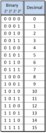
This adds up to fifteen and is represented in 4-bit binary shorthand as 1111. These two examples give the full range of a 4-bit binary number: An integer from zero to fifteen.

Here is the table of 4-bit binary-to-decimal conversions.

Model digitisation of a continuous graph into 4-bit binary

In order to model digitisation of a continuous graph, the following steps should suffice.

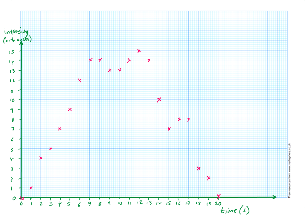
• Step 1: Draw a random graph, 20 data points long, with the y-axis between 0 and 15, like this one:

• Step 2: For each integer value on the x-axis, assign to the y-value the closest integer to the actual data point, like the pink data points here and in the following table:

Time (s)	Intensity (arb. Units)
0	0
1	1
2	4
3	5
4	7
5	9
6	12
7	14
8	14
9	13
10	13
11	14
12	15
13	14
14	10
15	7
16	8
17	8
18	3
19	2
20	0

• Step 3: Convert the y-values to 4-bit binary, perhaps using the conversion table given earlier:

Time (s)	Intensity (arb. Units)	Intensity (4-bit binary)
0	0	0000
1	1	0001
2	4	0100
3	5	0101
4	7	0111
5	9	1001
6	12	1100
7	14	1110
8	14	1110
9	13	1101
10	13	1101
11	14	1110
12	15	1111
13	14	1110
14	10	1010
15	7	0111
16	8	1000
17	8	1000
18	3	0011
19	2	0010
20	0	0000

• Step 4: Pass the 4-bit binary data to your work partner and take theirs from them:

Intensity (4-bit binary)
0000
0001
0100
0101
0111
1001
1100
1110
1101
1101
1110
1110
1111
1110
1010
0111
1000
1000
0011
0010
0000

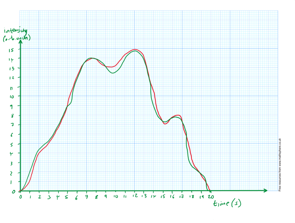
• Step 5: Convert the 4-bit binary y-values of your work partner back into integers and plot them on a graph, like the pink points here:

• Step 6: Reconstruct the graph by drawing a line of best fit through the data points, like this:

Step 7: Compare the reconstructed graph with the original:

So, in one simple sequence, you have modelled how to convert base-10 data numbers into 4-bit binary, encoded a graph, and decoded someone else’s graph.

If any pupils say that it is not perfect, you could point out that you can:

• Increase the sample rate. Increase the number of data points, e.g., one every 0.5 seconds
• Increase the bit depth. Increase the number of bits for the y-axis, e.g., 5-bit would allow 32 different y-values instead of only 16

Now set the pupils off to do their own examples.

Model converting a simple word into 8-bit binary

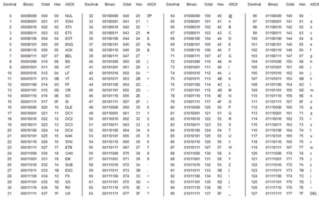
Now that conversion to binary is understood, we can increase the complexity. Roman characters each have a numerical value associated with them through the ASCII character map. If we can write letters as numerical values, we can write them in binary. It turns out for the ASCII map we want to use 8-bit binary, and the conversion chart is here (ignore the octal and hex columns):

Now the fun really starts. Let’s say I wanted to write “Hello” in binary, I start by writing the decimal number for each character from the character map:

H = 72, e = 101, l = 108, l = 108, o = 111.

Next, I convert each number into 8-bit binary (the conversion table given above can be used for this). As an example with the capital “H,” it’s character map position of 72 is equal to 64 + 8, which in 8-bit binary is:

(0x128) + (1x64) + (0x32) + (0x16) + (1x8) + (0x4) + (0x2) + (0x1)

Or, in shorthand, 01001000.

Repeating the above for the entire message, you get:

01001000 01100101 01101100 01101100 01101111

Summary

So, there is a standalone lesson on digitisation of data and of text.

The pupils learn something new and it can be incredibly fun, especially when they are sending messages to each other. In fact, one time, I received an extensive email from a pupil during the holidays, all written in 8-bit binary, just to tell me how much she had enjoyed it.

What’s also nice is you can squeeze it into half an hour or you can extend it to beyond an hour, depending on your own context.

Ultimately:

01010000 01101000 01111001 01110011 01101001 01100011 01110011 00100000 01101001 01110011 00100000 01100110 01110101 01101110 00100001

The 4-bit binary table is here and the 8-bit/ASCII table is here.